VLOOKUP, HLOOKUP, and XLOOKUP
VLOOKUP
The VLOOKUP stands for Vertical Lookup, this function is used to search for a specific value in the first column of a table and retrieve data from a different column in the same row. It’s ideal for scenarios where data is organized in columns, such as an inventory list, customer database, or price list.
Syntax:
=VLOOKUP(lookup_value, table_array, col_index_num, [range_lookup])
- lookup_value: The value you want to search for. This could be a specific text string, number, or reference to a cell that contains the value.
- table_array: The range of cells that contains the data, where the first column must contain the lookup value.
- col_index_num: The column number in the table array from which to return the result. The first column is 1, the second is 2, and so on.
- range_lookup: Optional. Use FALSE for an exact match (recommended for accurate results) or TRUE for an approximate match (useful for ranges or intervals).
Use Case:
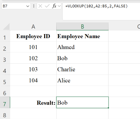
Imagine you have a table of Employee IDs and Employee Names and want to find the name of the employee with ID 102.
=VLOOKUP(102, A2:B10, 2, FALSE)

Explanation
- lookup_value is 102, the ID you’re looking up.
- table_array is A2:B10, the range containing both Employee IDs and Names.
- col_index_num is 2, meaning you want to return the value from the second column in the range (Employee Name).
- range_lookup is FALSE, ensuring an exact match (useful if Employee IDs are unique).
Notes
- VLOOKUP searches vertically, meaning it looks down the first column of the table until it finds the lookup value.
- If the lookup value isn’t found and you’re using FALSE for range_lookup, VLOOKUP will return #N/A.
- Limitation: VLOOKUP cannot look to the left. The lookup column must always be the first column in the specified range.
HLOOKUP
The HLOOKUP stands for Horizontal Lookup. It works similarly to VLOOKUP, but instead of searching vertically down a column, it searches horizontally across the first row. HLOOKUP is useful for tables where data is organized in rows rather than columns, such as a sales report by month or a schedule by week.
Syntax:
=HLOOKUP(lookup_value, table_array, row_index_num, [range_lookup])
- lookup_value: The value you want to search for in the first row.
- table_array: The range of cells that contains the data, where the first row must contain the lookup value.
- row_index_num: The row number within the table array from which to return the result. The first row is 1, the second is 2, and so on.
- range_lookup: Optional. Use FALSE for an exact match (recommended) or TRUE for an approximate match.
Use Case:
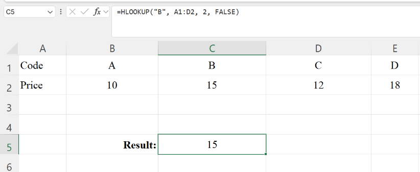
Suppose you have a table of Product Codes in the first row and their corresponding Prices in the second row. To find the price of Product B:
=HLOOKUP("B", A1:D2, 2, FALSE)

Explanation
- lookup_value is "B", the product code you’re looking up.
- table_array is A1:D2, the range covering both Product Codes and Prices.
- row_index_num is 2, indicating you want the result from the second row in the range (Price).
- range_lookup is FALSE, requiring an exact match.
Notes
- HLOOKUP searches horizontally, meaning it looks across the first row until it finds the lookup value.
- Like VLOOKUP, if the value isn’t found and FALSE is specified, it returns #N/A.
- Limitation: HLOOKUP only looks horizontally and does not support searching in other rows.
XLOOKUP
XLOOKUP is a powerful and flexible lookup function available in Excel 2019 and Microsoft 365. It overcomes many limitations of VLOOKUP and HLOOKUP by allowing bidirectional searching, supporting exact matches by default, and eliminating the need to count columns or rows manually. XLOOKUP can search both vertically and horizontally, making it a versatile choice for finding values in a range.
Syntax:
=XLOOKUP(lookup_value, lookup_array, return_array, [if_not_found], [match_mode], [search_mode])
- lookup_value: The value you want to search for.
- lookup_array: The range containing the value you want to search for.
- return_array: The range containing the value to return.
- if_not_found: Optional. A value to return if the lookup value is not found.
-
match_mode: Optional. Specifies the type of match:
- 0 for exact match (default).
- -1 for exact match or next smallest item.
- 1 for exact match or next largest item.
- 2 for wildcard match.
-
search_mode: Optional. Controls the direction of the search:
- 1 for search from first to last (default).
- -1 for search from last to first.
Use Case:
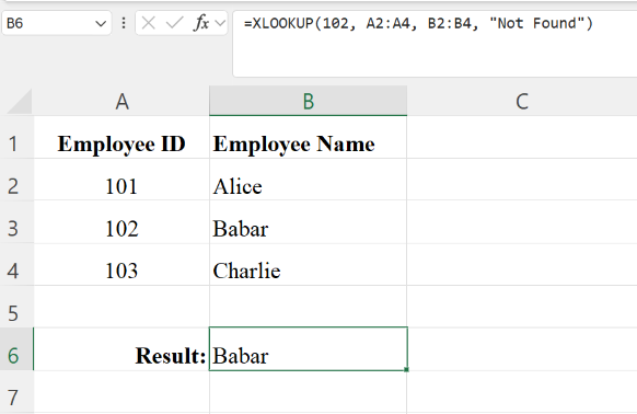
Using the same Employee ID and Employee Name table, if you want to find the employee name for ID 102, but want to specify "Not Found" if it’s missing:

Explanation
- lookup_value is 102, the value you’re searching for.
- lookup_array is A2:A10, the range containing Employee IDs.
- return_array is B2:B10, the range containing Employee Names.
- if_not_found is "Not Found", so this message will display if no match is found.
- match_mode and search_mode are not specified, so it defaults to exact match and first-to-last search order.
Key Advantages
- Bidirectional Search: XLOOKUP can search left-to-right, right-to-left, top-to-bottom, and bottom-to-top.
- Error Handling: if_not_found provides a way to handle missing data gracefully.
- Exact Match by Default: Unlike VLOOKUP and HLOOKUP, XLOOKUP performs exact matching by default, reducing errors.
Notes:
- Wildcard Search: Use * to match any number of characters and ? to match a single character (if match_mode is 2).
- More Flexible Range Selection: XLOOKUP doesn’t require the lookup and return arrays to be contiguous.
Summary Table
| Function | Search Direction | Use Case | Exact Match (default) |
|---|---|---|---|
| VLOOKUP | Vertical | When data is organized in columns | No |
| HLOOKUP | Horizontal | When data is organized in rows | No |
| XLOOKUP | Both Directions | Advanced search with error handling and flexibility | Yes |
Hands-On Assignment: Test Your Skills
In this assignment, you’ll use the VLOOKUP function to complete missing information on the "JourneyManagementPlan" sheet based on data from other sheets. The goal of this exercise is to help you understand the practical use of VLOOKUP in a real-world office scenario, where you will retrieve driver, vehicle, and passenger information from separate data sources.
Task 1: Driver's Details
- Emp. ID: Given as A001.
- Name: Use VLOOKUP to retrieve the name of the driver from the "StaffData" sheet based on the Emp. ID provided in cell C5.
- Driving License Number: Use VLOOKUP again to retrieve the driver's license number from the "StaffData" sheet using the Emp. ID in cell C5.
Task 2: Vehicle's Details
- Plate Number: Provided as A-12345.
- Make and Model: Use VLOOKUP to retrieve the make and model of the vehicle from the "VehiclesData" sheet based on the Plate Number in cell C10.
Task 3: Passenger's Details
- For each Emp. ID listed in the "Passenger's Details" section, use VLOOKUP to retrieve the Name and Designation of each passenger from the "StaffData" sheet.
Guidelines / Instructions
Referring to other sheets using a formula is simple if you understand and tricky as well, follow the steps mentioned below to have a better understanding.
The VLOOKUP Function comprises of Lookup Value, Table Array, Column Index Number and Range Lookup, after selecting each value add a comma "," to go for other values.
- Lookup Value: is the value to be used to search the data, in this assignment the value to search the data is Emp. ID from StaffData sheet and Plate Number from VehicleData Sheet.
- Table Array: is the range of data where you want to search for your Lookup Value, after the Lookup Value add a comma "," and click on the targeted sheet i.e. StaffData or VehicleData and select the range of data.
- Column Index Number: the first column is always the column of your Lookup Value that is number one 1 and if you are searching for Name then it is next to Emp. ID it means column number 2, so if you are searching for Name then column index will be 2 for Designation column number is 3 as it is the third column counting from the Emp. ID so the column index number will be 3 and so on.
- Range Lookup: There are 2 options (1)Approximate Match or (2)Exact Match, select Exact Match using the arrow keys to get the exact match of our Lookup Value, and press Enter to Tab Key to get the result.
Note: If a VLOOKUP formula returns an error (e.g., #N/A), it may mean that the Emp. ID or Plate Number is not found in the referenced range. Double-check the Emp. ID and Plate Number values or consider using IFERROR with VLOOKUP to display a custom message if the value is not found.
By completing this assignment, you’ll learn how to apply VLOOKUP to retrieve data from different sheets, which is a common requirement in office tasks where data is distributed across various sources.
Use of XLOOKUP Function
Now let's solve the same assignment using XLOOKUP Function, it comprises of Lookup value, Lookup Array, Return Array and If not found.
- Lookup value: similar to VLOOKUP and HLOOKUP, it is the value to be used to search the data.
- Lookup array: range of the data you want to search the Lookup value, by selecting the whole column (full column by clicking the column name at the top).
- Return array: select the whole column in which you are searching the end result for example in the assignment you will select Name, Driving License Number from StaffData and Make and Model from VehiclesData.
- If not found: insert text which to be displayed in case if the search result is not found, for example "Employee ID not found" this text will be displayed if the Lookup value is not found.
Summary:
All these Lookup Functions are extremely handy in practical, the XLOOKUP being the most flexible one, these useful functions are not limited to only same sheet or same workbook, but also be used to between different workbooks as well.
Submit Your Completed Assignment
Please save your completed assignment file, and email it to: assignments@muamlati.com