Introduction to Essential Excel Functions
Microsoft Excel is a powerful tool for handling data, performing calculations, and generating meaningful insights. This page is dedicated to helping you understand some of the most commonly used Excel functions that are crucial for both beginners and experienced users. These functions simplify a wide range of tasks, from basic summing and averaging of values to extracting specific text from cells.
Below are some of the most commonly used functions in Excel, which are fundamental for performing calculations and data analysis.
SUM Function
The SUM function adds together a range of numbers in Excel, instead of having the sum of cells using =A1+A2+A3 you can use SUM.
Syntax:
=SUM(number1, [number2], ...)
Use Case:
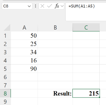
If you want to add the numbers in cells A1 to A5, the formula would be:
=SUM(A1:A5)
Explanation
So instead of =A1+A2+A3+A4+A5 just =SUM(A1:A5) will do the job, here ":" is used to denote a range of cells starting from A1 to A5
AVERAGE Function
The AVERAGE function calculates the average (mean) of a range of numbers, average formula is the TOTAL / COUNT so instead of first getting the sum of and then dividing them with the count the AVERAGE Function does it in easier and faster way.
Syntax:
=AVERAGE(number1, [number2], ...)
Use Case:
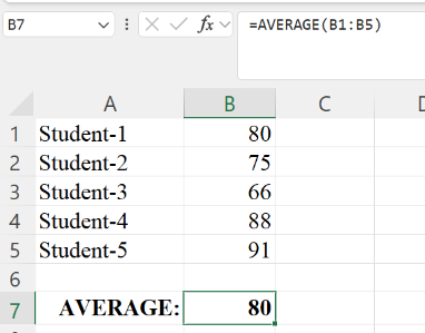
To find the average total marks scored by the students in a class.
=AVERAGE(B1:B5)
Explanation
The otherway to get the average was to first calculate the SUM of all the total marks and then divide the result by the total number of students. Using AVERAGE Function made it easy.
COUNT Function
The COUNT function counts the number of cells that contain numbers in a specified range.
Syntax:
=COUNT(value1, [value2], ...)
Use Case:
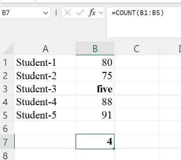
To count how many numeric entries exist in a data range. Lets take the example of previous case, apply the COUNT Function for cells B1 to B5
=COUNT(B1:B5)
Explanation
The result of =COUNT(B1:B5) is 4 because cell B3 contains text therefore that doesn't get counted.
COUNTA Function
The COUNTA function counts the number of cells that are not empty in a specified range, including text and numbers.
Syntax:
=COUNTA(value1, [value2], ...)
Use Case:
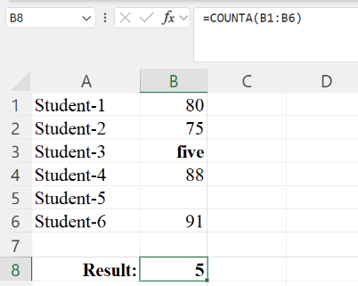
To count the number of non-empty cells in a data range.
=COUNTA(B1:B6)
Explanation
The result of =COUNTA(B1:B6) is 5 counted all the cells having text and numbers excluding cell B5 because it is empty.
MIN Function
The MIN function returns the smallest value in a range of numbers.
Syntax:
=MIN(number1, [number2], ...)
Use Case:
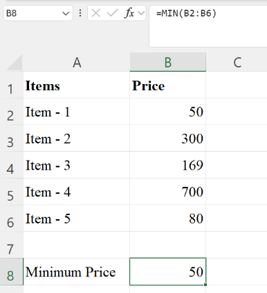
To quickly identify the minimum value in a data set. To find the smallest value in the range B2:B6.
=MIN(B2:B6)
Explanation
The result is 50 the minimum / lowest value in the range.
MAX Function
The MAX function returns the largest value in a range of numbers.
Syntax:
=MAX(number1, [number2], ...)
Use Case:
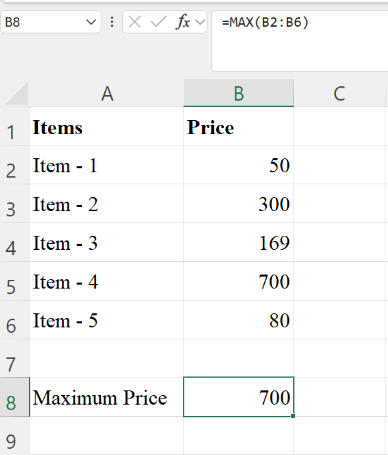
To quickly identify the maximum value in a data set. To find the largest value in the range B2:B6.
=MAX(B2:B6)
Explanation
The result is 7000 the maximum / largest value in the range.
MOD Function
The MOD function in Excel is a powerful yet often overlooked tool that allows you to find the remainder when one number is divided by another. This function is especially useful for calculations that involve grouping, periodicity, or checking even/odd values.
Syntax:
=MOD(number, divisor)
- number: The number you want to divide.
- divisor: The number by which you want to divide number to find the remainder.
Example:
When =MOD(10,3) will result 1, and = MOD(20,5) will result 0 (zero) .
Lets check out some of the basic functions used for characters.
LEFT Function
The LEFT function extracts a specified number of characters from the left side of a text string.
Syntax:
=LEFT(text, [num_chars])
Use Case:
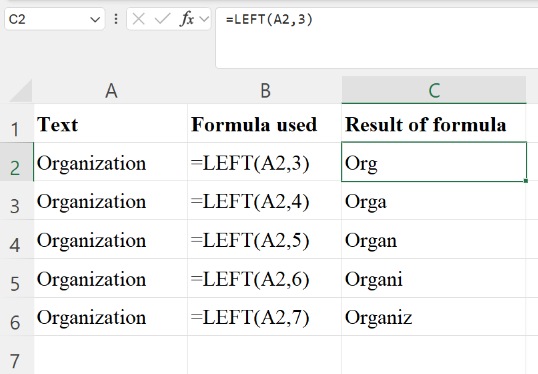
Use this function to extract a portion of a string, such as extracting the first few letters of a name or code. To extract the first 3 characters from cell A2.
=LEFT(A2, 3)
RIGHT Function
The RIGHT function extracts a specified number of characters from the right side of a text string.
Syntax:
=RIGHT(text, [num_chars])
Use Case:
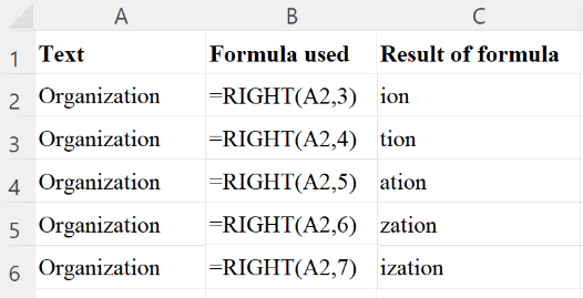
It is opposite of LEFT Function, Lets have the similar example of above by using RIGHT Function.
=RIGHT(A2, 3)
MID Function
The MID function extracts characters from the middle of a text string, based on a starting position and number of characters.
Syntax:
=MID(text, start_num, num_chars)
Use Case:
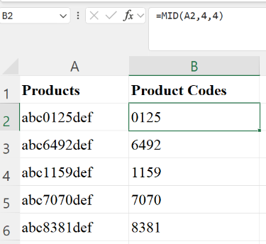
Use this function to extract a substring from the middle of a text, for instance, extracting specific parts of a product code.
=MID(A2,4,4)
- "A2": is the cell referred.
- A2,"4": starting position of characters to include.
- A2,4,"4": number of characters required in result.
LEN Function
The LEN function returns the length (number of characters) of a text string.
Syntax:
=LEN(text)
Use Case:
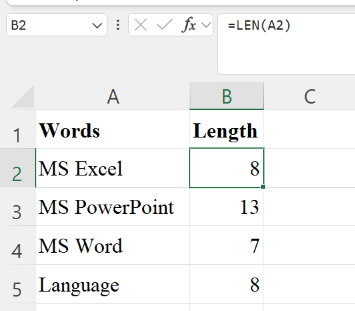
This is useful for counting the number of characters in a string, especially when cleaning or validating data, it also counts the spaces if any in the cell referred irrespective of the space location whether it is in the beginning or end.
=LEN(A2)
CONCATENATE Function
The CONCATENATE function (or & operator) joins two or more text strings into one.
Syntax:
=CONCATENATE(text1, [text2], ...)
Note: In newer versions of Excel, you can also use TEXTJOIN or the & operator.
Use Case:
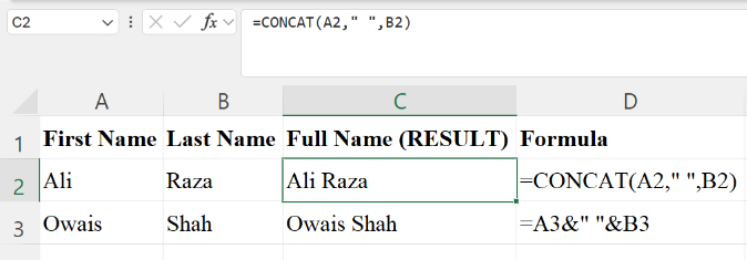
You can join multiple text strings, like combining first and last names, or creating a full product code.
=CONCATENATE(A2, " ", B2)
Or
=A3 & " " & B3
Hands-On Assignment: Test Your Skills
Now that you have good understanding of Essential Functions and also you have the knowledge of IF Functions then it is time for practical assignment.
Download Assignment - Sales Evaluation
Objective:
- Calculate Total Sales.
- Find the Highes Sales achieved in a month for each sales person.
- Find the Lowest Sales achieved in a month for each sales person.
- Calculate Average Sales.
- Evaluation Remarks.
Instructions:
- For all caculations use the Functions explained above.
- Evaluation Remarks: Company has set Yearly target of $ 150,000 for each sales person, so accordingly you have to find out:
- If Monthly Sales Average is less than the average of yearly target
150000 / 12 = 12500then Evaluation Remarks = "Improvement required to achieve yearly sales target". - If Monthly Sales Average is equal to or higher than average of yearly target then Evaluation Remarks = "On Track to achieve yearly sales target".
- Ensure that if the amount in sales are updated or changed, the results for all calcuations should update accordingly. This will verify if your formulas are correctly referencing the appropriate cells and ranges.
Submit Your Completed Assignment
Please save your completed assignment file, and email it to: assignments@muamlati.com